Getting Started
Welcome to EpiNexus! This guide will walk you through using the web interface to analyse your ChIP-seq, histone modification, or other epigenomic data — no command-line or coding experience needed.
How EpiNexus Works
Upload your files
Drag and drop your FASTQ.gz files — or upload BAM / BED / peak files — and choose your reference genome.
EpiNexus runs your analysis
A full epigenomic pipeline runs automatically — from raw QC to publication-ready results.
Explore interactive results
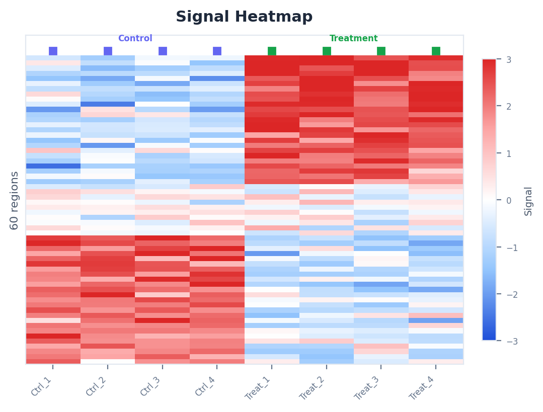
Browse volcano plots, heatmaps, super-enhancer rankings, and more — all interactive, all downloadable.
What you can do with EpiNexus
Check data quality
See mapping rates, duplication, FRiP scores and more for every sample.
Annotate peaks
Find out which genes and genomic features your peaks overlap.
Compare conditions
Identify peaks that are gained or lost between treatment and control.
Integrate marks
Combine H3K27ac + H3K27me3 to classify active, poised, and bivalent states.
Find super-enhancers
Detect large regulatory regions that drive cell identity genes.
Link peaks to genes
Connect enhancer peaks to their likely target genes.
Before you begin
You will need your data files ready to upload. EpiNexus accepts:
FASTQ files
Raw sequencing reads straight from the sequencer. If your data hasn't been aligned yet, start here — EpiNexus handles everything from raw reads onward.
BAM files
Aligned sequencing reads (already mapped to a genome). This is the most common starting point — your core facility usually provides BAM files after sequencing.
Peak files (optional)
If your core facility already called peaks (.narrowPeak, .broadPeak, or .bed), you can upload those alongside your BAM files. If not, EpiNexus calls peaks for you.
Once you have your files, follow the steps in the sidebar — starting with Create a Project.
Create a Project
A project is a container for one experiment — it groups your samples, analysis runs, and results together in one place.
Open the Projects page
Click Projects in the top navigation bar. You will see a list of any existing projects, or an empty state if this is your first time.
Click "New Project"
The blue + New Project button is in the top-right corner.
Fill in the details
Project name — Give it a descriptive name, e.g. “H3K27ac Treatment vs Control - March 2026”.
Description (optional) — Add notes about the experiment for your records.
Genome — Choose the reference genome your samples were aligned to. Common choices:
Many more organisms are available — see the full list on the Pipelines page. Not sure which genome? Check with whoever aligned your data, or look at the BAM file header. Most recent human data uses hg38.
Click "Create"
Your project is ready! You will be taken to the project page where you can upload files.
Tip: One project per experiment
Keep things organised by creating separate projects for different experiments. For example, one project for “H3K27ac in liver cancer” and another for “H3K4me3 in normal liver”.
Upload Your Files
After creating a project, you need to upload your sequencing data files. EpiNexus handles all the bioinformatics processing from there.
Open your project
Click on the project name from the Projects page to open it.
Go to the Files tab
You will see a file manager area with an upload zone. You can drag and drop files or click to browse.
Upload your sequencing files
Select the files for your experiment. Depending on what your core facility provided:
FASTQ files — Raw reads from the sequencer. Upload both read 1 and read 2 files for paired-end data.
BAM files — Aligned reads (most common). Each BAM file represents one sample (e.g. “Treatment_Rep1.bam”, “Control_Rep1.bam”).
Files upload in the background — you can see the progress bar for each one.
Upload peak files (optional)
If your facility also provided peak calls (.narrowPeak or .broadPeak files), upload those alongside your BAM files. Name them to match — e.g. “Treatment_Rep1.narrowPeak” alongside “Treatment_Rep1.bam”. EpiNexus will automatically pair them. If you don't have peak files, EpiNexus calls peaks for you.
Wait for uploads to finish
All files must finish uploading before you start an analysis. A green checkmark appears next to each completed file.
How big are these files?
| File type | Typical size | What it contains |
|---|---|---|
| FASTQ | 5 – 30 GB | Raw sequencing reads straight from the sequencer |
| BAM | 1 – 10 GB | Aligned sequencing reads mapped to the genome |
| narrowPeak | 0.5 – 5 MB | Regions where your histone mark is enriched (sharp peaks) |
| broadPeak | 1 – 20 MB | Regions where your histone mark is enriched (broad domains) |
Large file tip
BAM and FASTQ files can be very large. We recommend a stable internet connection. If an upload is interrupted, you can simply re-upload the same file — it will resume or replace the partial upload.
Run an Analysis
Once your files are uploaded, you can launch an analysis run. EpiNexus will automatically detect your files and run the appropriate analysis steps.
Click "New Run"
From your project page, click the + New Run button.
Name your run
Give it a recognisable name like “Initial analysis” or “H3K27ac differential”. You can run the same project multiple times with different settings.
Choose a pipeline
EpiNexus offers three pipelines depending on your starting data:
Full pipeline
Start here if you have FASTQ files. Runs alignment, peak calling, QC, annotation, differential analysis, integration, and super-enhancers — everything from raw reads to results.
Preprocessing pipeline
Also for FASTQ files, but only runs the preprocessing steps (alignment, filtering, peak calling) without the downstream analysis. Useful if you just need BAM and peak files.
Analysis pipeline
Start here if you have BAM files (and optionally peak files). Runs QC, annotation, differential, integration, and super-enhancer detection.
Not sure? If your core facility gave you FASTQ files, choose Full. If they gave you BAM files, choose Analysis.
Review settings (or keep defaults)
The defaults work well for most experiments. You can adjust parameters if needed — see Settings & Options for details.
Click "Run"
The analysis starts immediately. You can close the browser and come back later — the analysis runs on the server and will complete in the background.
Watching progress
While the analysis is running, you will see a progress bar and the current step name. A typical analysis of 4–6 BAM samples takes 5–15 minutes. If you start from FASTQ files, preprocessing (alignment and peak calling) runs first and takes longer (typically 2–8 hours depending on assay and sequencing depth). If preprocessing fails, the downstream analysis steps cannot proceed. The downstream analysis steps (QC, annotation, differential, super-enhancers) run independently of each other, so a failure in one does not block the others.
View Results
When the analysis finishes, EpiNexus presents your results in an interactive dashboard. Click on a completed run to open the results.
Results overview
The results page shows a summary at the top with key numbers: how many peaks were found, how many are significant, how many samples passed QC. Below that, you can navigate to individual result sections:
Quality Control
A table showing metrics for each sample: total reads, mapping rate, duplicate rate, FRiP score (fraction of reads in peaks), and whether each sample passed QC thresholds. Samples with low FRiP or high duplication are flagged with warnings.
Peak Annotations
A browsable table of all peaks annotated with their nearest gene, distance to the transcription start site (TSS), and genomic feature (promoter, exon, intron, or intergenic). You can sort and filter by gene name or feature type.
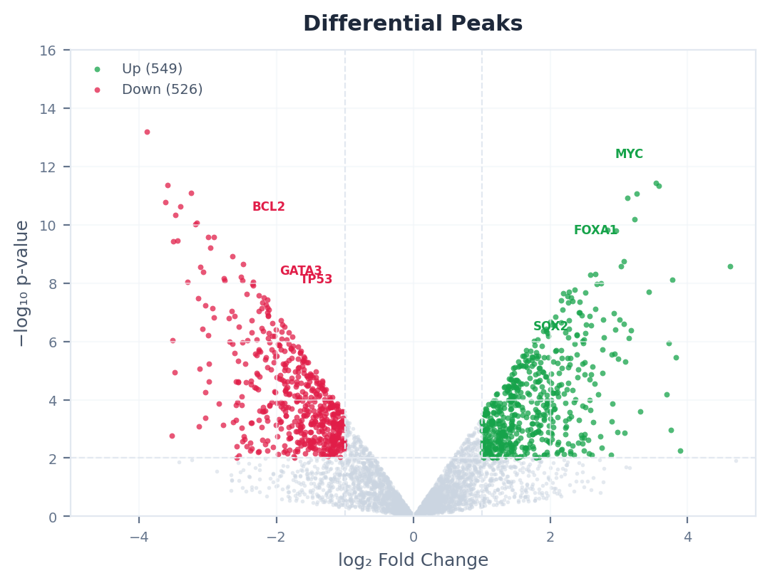
Differential Peaks
Peaks that change significantly between your conditions. Shown as a table with fold-change, significance (FDR), and direction (gained or lost). Filter by chromosome or direction to find peaks near your genes of interest.
Multi-Mark Integration
If you analysed more than one histone mark (e.g. H3K27ac and H3K27me3), this section shows the chromatin state classification: which genes are active, poised, bivalent, or repressed, and which genes switch states between conditions.
Super-Enhancers
Large regulatory elements identified by the ROSE algorithm. The table shows each super-enhancer’s location, signal strength, rank, and the nearest gene. Super-enhancers are often associated with cell-identity genes and disease drivers.
Peak–Gene Links
Connections between enhancer peaks and their predicted target genes, based on genomic distance or the Activity-by-Contact (ABC) model. Useful for understanding which enhancers regulate which genes.
Understand Your Data
Not sure what these results mean? Here is a plain-language guide to the key concepts.
What is a “peak”?
A peak is a region of the genome where your histone mark is enriched compared to the background. Think of it as a “hotspot” of epigenetic activity. Each peak has a location (chromosome, start, end) and a signal strength.
What is FRiP score?
Fraction of Reads in Peaks — what percentage of your sequencing reads land inside called peaks. Higher is better. A FRiP above 1% is the ENCODE minimum; above 5% is good; above 20% is excellent. Low FRiP may mean low enrichment or too much background.
What does “differential” mean?
A differential peak is one that is significantly more (gained) or less (lost) enriched in one condition versus another. For example, an H3K27ac peak that appears only in treated cells but not in control cells is a “gained” peak — suggesting that genomic region became activated by the treatment.
What is FDR?
False Discovery Rate — the probability that a result is a false positive. An FDR of 0.05 means there is a 5% chance this peak is not truly different between conditions. Lower FDR = more confident. The default threshold is 0.1 (10%).
What is a super-enhancer?
Super-enhancers are clusters of nearby enhancers that have unusually high levels of histone modification signal (typically H3K27ac). They control important cell-identity genes and are often disrupted in cancer. They are identified by ranking all enhancer regions by signal and finding the “inflection point” above which regions are exceptionally strong.
What are bivalent domains?
Regions of the genome that carry both an activating mark (like H3K4me3) and a repressive mark (like H3K27me3) at the same time. These genes are “poised” — ready to be quickly switched on or off. Bivalent domains are especially important in stem cells and development.
What does “distance to TSS” mean?
TSS = Transcription Start Site, the beginning of a gene. The distance from a peak to the nearest TSS helps you understand whether a peak is at a promoter (close to TSS, within ~3 kb) or at a distal enhancer (far from TSS, often 10–1000 kb away).
Settings & Options
The default settings work well for most histone ChIP-seq experiments. If you need to fine-tune the analysis, here are the options available when launching a run:
| Setting | Default | What it does |
|---|---|---|
| Genome | hg38 | The reference genome your data was aligned to. Make sure this matches your BAM files. |
| TSS window | ± 3,000 bp | How far from a gene’s start site a peak can be and still count as “promoter”. The default of 3 kb upstream and downstream is standard for most analyses. |
| FDR threshold | 0.1 | The significance cutoff for differential peaks. Lower values (e.g. 0.05) are more stringent — fewer peaks but higher confidence. |
| Fold-change threshold | 0.5 | Minimum log2 fold-change for a peak to be called differential. Higher values only report large changes. |
| Enhancer stitching distance | 12,500 bp | How close two enhancer peaks need to be to get merged into one super-enhancer candidate. The 12.5 kb default matches the original ROSE paper. |
| Peak–gene max distance | 1,000,000 bp | Maximum distance between a peak and a gene for them to be linked. 1 Mb is a common default for enhancer-gene associations. |
When should I change the defaults?
For most experiments, the defaults are fine. Consider changing the FDR threshold if you are getting too many or too few differential peaks. If you are studying very broad histone marks (like H3K27me3 or H3K9me3), a larger TSS window might be appropriate.
Troubleshooting
My analysis failed
Check the run details for error messages. The most common causes are: (1) wrong genome selected — make sure your files match the chosen reference, (2) corrupted or truncated upload — try re-uploading, (3) very low quality data with no peaks detected. If none of these apply, reach out via the Contact page.
Upload is stuck or timing out
Large FASTQ.gz files can take several minutes to upload depending on your connection. If the upload fails, check that each file is under the size limit and that your browser tab stays open during the transfer. Splitting very large files before upload can also help.
No peaks detected
This usually means the data has very low signal-to-noise. Verify that (1) the correct assay type is selected, (2) you have enough sequencing depth (at least 10–20M reads for ChIP-seq), and (3) the antibody or enrichment step worked as expected. Check the QC report for library complexity and FRiP scores.
Differential analysis shows zero results
Make sure you have at least two conditions with replicates. If you only have one sample per condition, the statistical test cannot estimate variance. Also check that the correct comparisons are set up — EpiNexus compares the groups exactly as you define them.
Results look different from my previous tool
Minor differences in peak counts or differential calls are expected between tools due to different default parameters (e.g. FDR threshold, minimum fold-change). Check the Settings & Options section above to adjust these parameters. For peak calling, EpiNexus uses MACS2 for ChIP-seq and ATAC-seq, and SEACR for CUT&Tag and CUT&Run.
Browser is slow or unresponsive
Interactive plots with very large datasets (>100k peaks) can be demanding. Try using Chrome or Firefox with hardware acceleration enabled. Closing other tabs can also free up memory. If a specific plot is slow, use the built-in filters to reduce the data shown.
I cannot delete a project
Go to the Projects page, find the project, and click the trash icon. You will be asked to confirm. Note that deletion is permanent — all uploaded files and results will be removed. If the button is greyed out, the project may still have a running analysis; wait for it to finish first.